Pay Discrimination Analysis

This is an AM01 Applied statitics project undertaken by my study group to analyse the pay differences among men and women. We have analysed the relationship between salary and gender via visualisation and hypothesis testing. We have also determined reltionship between experience and gender along with salaty & experience for the pool of men and women in our dataset. We have also calculated correlation between gender, experience and salaries to draw final inferences from out data.
Omega Group- Pay Discrimination
Objective: Find out whether there is indeed a significant difference between the salaries of men and women, and whether the difference is due to discrimination or whether it is based on another, possibly valid, determining factor.
Loading the data:
omega <- read_csv(here::here("data", "omega.csv"))
glimpse(omega) # examine the data frame
## Rows: 50
## Columns: 3
## $ salary <dbl> 81894, 69517, 68589, 74881, 65598, 76840, 78800, 70033, 635…
## $ gender <chr> "male", "male", "male", "male", "male", "male", "male", "ma…
## $ experience <dbl> 16, 25, 15, 33, 16, 19, 32, 34, 1, 44, 7, 14, 33, 19, 24, 3…Analysis of Relationship between Salary & Gender
# Summary Statistics of salary by gender
kable(favstats (salary ~ gender, data=omega))| gender | min | Q1 | median | Q3 | max | mean | sd | n | missing |
|---|---|---|---|---|---|---|---|---|---|
| female | 47033 | 60338 | 64618 | 70033 | 78800 | 64543 | 7567 | 26 | 0 |
| male | 54768 | 68331 | 74675 | 78568 | 84576 | 73239 | 7463 | 24 | 0 |
# Dataframe with two rows (male-female) and having as columns gender, mean, SD, sample size,
# the t-critical value, the standard error, the margin of error,
# and the low/high endpoints of a 95% condifence interval

ci_omega <- omega %>%
  group_by(gender) %>%
  summarize(mean = mean(salary, na.rm=TRUE),
            sd = sd(salary, na.rm=TRUE),
            count = n(),
            t_critical = qt(0.975, count-1),
            se_diff = sd/sqrt(count),
            margin_of_error = t_critical * se_diff,
            salary_low = mean - margin_of_error,
            salary_high = mean + margin_of_error)

# print the table with confidence interval

kable(ci_omega,
caption="Salary CI by Gender")| gender | mean | sd | count | t_critical | se_diff | margin_of_error | salary_low | salary_high |
|---|---|---|---|---|---|---|---|---|
| female | 64543 | 7567 | 26 | 2.06 | 1484 | 3056 | 61486 | 67599 |
| male | 73239 | 7463 | 24 | 2.07 | 1523 | 3151 | 70088 | 76390 |
Inference:
The two confidence interval for women and men salary of a 95% do not overlap. The difference in salary between the two groups is thus significantly different. The t-test would thus not be needed in this case.
Analysis of relationship between salary & gender via Hypothesis Test (t.test + infer)
# hypothesis testing using t.test()

t.test(salary ~ gender, data = omega)
##
## Welch Two Sample t-test
##
## data: salary by gender
## t = -4, df = 48, p-value = 0.0002
## alternative hypothesis: true difference in means between group female and group male is not equal to 0
## 95 percent confidence interval:
## -12973 -4420
## sample estimates:
## mean in group female mean in group male
## 64543 73239# hypothesis testing using infer package
#Calculating observed statistic
obs_stat <- omega %>%
specify(salary ~ gender) %>%
calculate(stat = "diff in means",
order = c("female", "male"))
set.seed(1234)
salaries_in_null_world <- omega %>%
#Which variable we are interested in
specify(salary ~ gender) %>%
#Hypothesis with no (null) difference
hypothesize(null = "independence") %>%
#Create simulated samples
generate(reps = 10000, type = "permute") %>%
#Mean difference in each sample
calculate(stat = "diff in means",
order = c("female", "male")) # give the order for subtraction first, second
#Visualize distribution
salaries_in_null_world %>% visualize()+
shade_p_value(obs_stat = obs_stat, direction = "both") 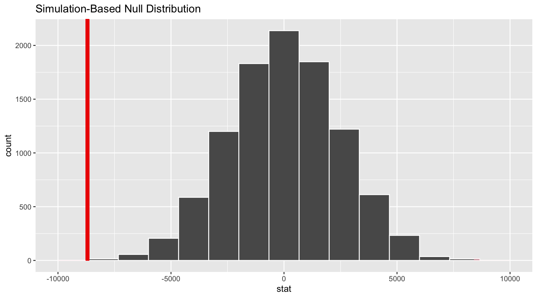
salaries_in_null_world %>%
  get_p_value(obs_stat = obs_stat, direction = "both")
## # A tibble: 1 × 1
## p_value
## <dbl>
## 1 0.0002Inference:
The R t-test clearly showed that the null hypothesis (no difference) can be rejected. This can be seen by three indicators: first the |t-stat| is approximately > 2, second the CI for delta does not contain zero, third the p-value is < 5%.
With 1000 reps the bootstrap simulation gave a p-value of zero, this can be the case when the observed statistic is very unlikely. We thus had to increase the reps to 10000 to replicate the results from the formula.
Analysis of relationship between experience & gender:
# Summary Statistics of salary by gender
favstats (experience ~ gender, data=omega)
## gender min Q1 median Q3 max mean sd n missing
## 1 female 0 0.25 3.0 14.0 29 7.38 8.51 26 0
## 2 male 1 15.75 19.5 31.2 44 21.12 10.92 24 0Based on this evidence, can you conclude that there is a significant difference between the experience of the male and female executives? Does your conclusion validate or endanger your conclusion about the difference in male and female salaries?
#Using formula to create confidence interval

ci_omega_experience <- omega %>%
  group_by(gender) %>%
  summarize(mean = mean(experience, na.rm=TRUE),
            sd = sd(experience, na.rm=TRUE),
            count = n(),
            t_critical = qt(0.975, count-1),
            se_diff = sd/sqrt(count),
            margin_of_error = t_critical * se_diff,
            experience_low = mean - margin_of_error,
            experience_high = mean + margin_of_error)

# print the table with confidence interval

kable(ci_omega_experience,
caption="Experience CI by Gender")| gender | mean | sd | count | t_critical | se_diff | margin_of_error | experience_low | experience_high |
|---|---|---|---|---|---|---|---|---|
| female | 7.38 | 8.51 | 26 | 2.06 | 1.67 | 3.44 | 3.95 | 10.8 |
| male | 21.12 | 10.92 | 24 | 2.07 | 2.23 | 4.61 | 16.52 | 25.7 |
Answer:
The two experience confidence intervals for women and men at 95% do not overlap. The difference between the two groups is thus significantly different and there is no need to run a t-test. These findings would endager the conclusion drawn above (gender-based salary discrimination) as it seems that not only gender, but an additional previously not considered factor, experience, could influence the pay-gap. Further anaylsis is suggested.
Analysis of relationship between salary & experience:
Someone at the meeting argues that clearly, a more thorough analysis of the relationship between salary and experience is required before any conclusion can be drawn about whether there is any gender-based salary discrimination in the company.
Analyse the relationship between salary and experience. Draw a scatterplot to visually inspect the data
ggplot(omega, aes(x = experience, y = salary, color = gender)) +
  geom_point()+
  geom_smooth(method='lm', se=FALSE)+
  labs(
    title = "Relationship between salary and experience"
  )+
  theme_bw()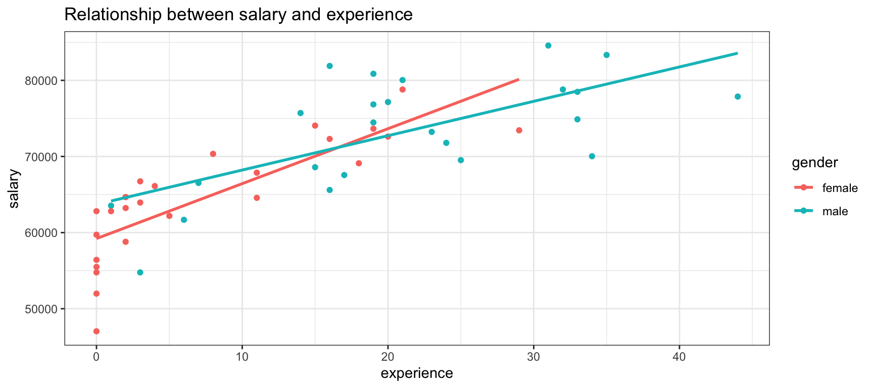
Correlations between Gender, Experience and Salary
omega %>%
  select(gender, experience, salary) %>% #order variables they will appear in ggpairs()
  ggpairs(aes(colour=gender, alpha = 0.3))+
  theme_bw()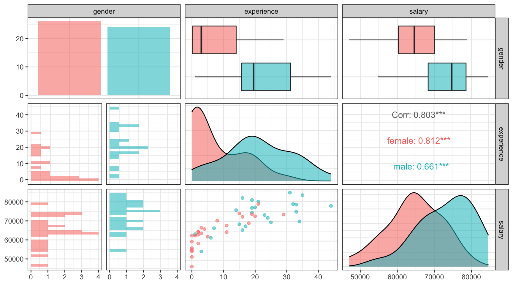
Inference:
The correlation matrix reweals many interesting things in just one visualization. Looking at the scatterplot we can see a clear correlation between years of experience and salary, this is true for both genders. The correlation can also be confirmed mathematically with a total cor of 0.8. In other words, the higher the experience the higher the salary. We have used two colors in the plot above to demonstrate that women salary increase more significantly with growing experience (stepper slope). With women having a median experience of 3 and men of 19.5 it is thus not surprising that there is a significant pay-gap. Omega should rather investigate the underlying reason why women have so little work experience. Are senior positions which require more experience mainly filled by man while graduate positions mainly by women? Anyhow, further investigation is needed!