Health pattern analysis

This is an AM01 Applied statitics project undertaken by my study group to analyse the Youth Risk Behavior Surveillance data to study health pattern among high school students. We have performed EDA on YRBSS data to gain insights on the weight data available for high school students. We have also done analysis of physically active people in addition to determining confidence interval for inactive students.We have also plotted graphs to understand the relationship between physical activity and weight among the students.
About: Youth Risk Behavior Surveillance
Every two years, the Centers for Disease Control and Prevention conduct the Youth Risk Behavior Surveillance System (YRBSS) survey, where it takes data from high schoolers (9th through 12th grade), to analyze health patterns. You will work with a selected group of variables from a random sample of observations during one of the years the YRBSS was conducted.
Exploratory Data Analysis on distribution of weight data
data(yrbss)

# Create summary statistics
summary(yrbss$weight)
## Min. 1st Qu. Median Mean 3rd Qu. Max. NA's
## 30 56 64 68 76 181 1004skimr::skim(yrbss)| Name | yrbss |
| Number of rows | 13583 |
| Number of columns | 13 |
| _______________________ | |
| Column type frequency: | |
| character | 8 |
| numeric | 5 |
| ________________________ | |
| Group variables | None |
Variable type: character
| skim_variable | n_missing | complete_rate | min | max | empty | n_unique | whitespace |
|---|---|---|---|---|---|---|---|
| gender | 12 | 1.00 | 4 | 6 | 0 | 2 | 0 |
| grade | 79 | 0.99 | 1 | 5 | 0 | 5 | 0 |
| hispanic | 231 | 0.98 | 3 | 8 | 0 | 2 | 0 |
| race | 2805 | 0.79 | 5 | 41 | 0 | 5 | 0 |
| helmet_12m | 311 | 0.98 | 5 | 12 | 0 | 6 | 0 |
| text_while_driving_30d | 918 | 0.93 | 1 | 13 | 0 | 8 | 0 |
| hours_tv_per_school_day | 338 | 0.98 | 1 | 12 | 0 | 7 | 0 |
| school_night_hours_sleep | 1248 | 0.91 | 1 | 3 | 0 | 7 | 0 |
Variable type: numeric
| skim_variable | n_missing | complete_rate | mean | sd | p0 | p25 | p50 | p75 | p100 | hist |
|---|---|---|---|---|---|---|---|---|---|---|
| age | 77 | 0.99 | 16.16 | 1.26 | 12.00 | 15.0 | 16.00 | 17.00 | 18.00 | ▁▂▅▅▇ |
| height | 1004 | 0.93 | 1.69 | 0.10 | 1.27 | 1.6 | 1.68 | 1.78 | 2.11 | ▁▅▇▃▁ |
| weight | 1004 | 0.93 | 67.91 | 16.90 | 29.94 | 56.2 | 64.41 | 76.20 | 180.99 | ▆▇▂▁▁ |
| physically_active_7d | 273 | 0.98 | 3.90 | 2.56 | 0.00 | 2.0 | 4.00 | 7.00 | 7.00 | ▆▂▅▃▇ |
| strength_training_7d | 1176 | 0.91 | 2.95 | 2.58 | 0.00 | 0.0 | 3.00 | 5.00 | 7.00 | ▇▂▅▂▅ |
# Plot missing values
kable(yrbss%>%
  filter(is.na(weight))%>%
summarise(Tatal_missing_data=n()),"simple")| Tatal_missing_data |
|---|
| 1004 |
# Create histogram
x <- yrbss$weight
h<-hist(x,
xlab="weight", main="Histogram with Normal Curve")
# Create normal distribution as comparison
xfit<-seq(min(x,na.rm = TRUE),max(x,na.rm = TRUE),length=40) # order the data
yfit<-dnorm(xfit,mean=mean(x,na.rm = TRUE),sd=sd(x,na.rm = TRUE)) # density of normal dis
yfit <- yfit*diff(h$mids[1:2])*length(x)
lines(xfit, yfit, col="red", lwd=2) 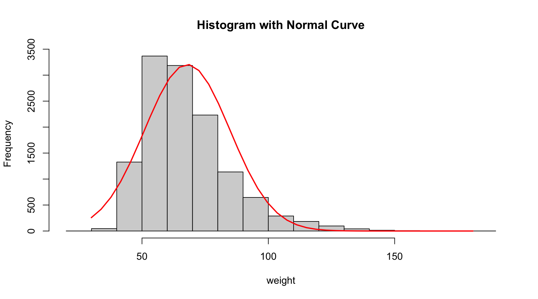 Inference:
The minimum value of weight is 30, the maximum value is 181, the median is 64, the lower quantile is 56, the upper quantile is 76, and the total number of missing values is 1004. The distribution of weights looks lightly skewed to the right. We added a normal distribution line as comparison.
Analysis of physically active people (>3 days a week):
# Create new variable
yrbss$physical_3plus<-ifelse(yrbss$physically_active_7d>=3,"yes","no")

# Method group_by()... summarise()
yrbss%>%
  group_by(physical_3plus)%>%
  summarise(n=n())%>%
  mutate(prop=label_percent()(n/nrow(yrbss)))
## # A tibble: 3 × 3
## physical_3plus n prop
## <chr> <int> <chr>
## 1 no 4404 32%
## 2 yes 8906 66%
## 3 <NA> 273 2%# Method count()
yrbss%>%
count(physical_3plus) %>%
mutate(prop=label_percent()(n/nrow(yrbss)))## # A tibble: 3 × 3
## physical_3plus n prop
## <chr> <int> <chr>
## 1 no 4404 32%
## 2 yes 8906 66%
## 3 <NA> 273 2%# Create a graph to show difference
yrbss%>%
filter(is.na(physical_3plus)==FALSE)%>%
group_by(physical_3plus)%>%
summarise(number=n())%>%
ggplot(aes(x=physical_3plus,y=number))+
geom_bar(stat = "identity",width =0.5)+
labs(x="physical_3plus",y="number")+
ggtitle("How many children workout 3plus times?",
subtitle = "")+
theme_bw()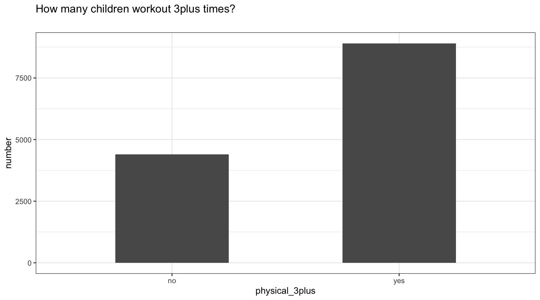 Inference:
In this first analysis we have separately shown the percentage proportion also for the NA values. 8906 kids practice sport 3plus times a week while 4404 do not. In the graph we have not included the NA values.
Confidence Interval calculation for the population proportion of high schools that are NOT active 3 or more days per week
#Filtering data

test<-yrbss %>%
  filter(is.na(physical_3plus)==FALSE)%>%

# Changing yes no to numerical value to make it easier
  mutate(physical_3_p=ifelse(physical_3plus=="yes",1,0), physical_3_l=ifelse(physical_3plus=="no",1,0))


# With formula

ci_yrbss <- test %>%
  filter(!is.na(physical_3plus)) %>%
  summarize(count = n(),
            p = (sum(physical_3plus == "no"))/count,
            t_critical = qt(0.975, count-1),
            se_diff = sqrt(p*(1-p)/count),
            margin_of_error = t_critical * se_diff,
            prop_low = p - margin_of_error,
            prop_high = p + margin_of_error)

# print the table with confidence interval

kable(ci_yrbss,
caption="CI 3 or more times active Formula")| count | p | t_critical | se_diff | margin_of_error | prop_low | prop_high |
|---|---|---|---|---|---|---|
| 13310 | 0.331 | 1.96 | 0.004 | 0.008 | 0.323 | 0.339 |
# Confidence Interval with bootstrap

set.seed(1234)
boot_3lower <- test %>%
# Select
  filter(is.na(physical_3plus)==FALSE)%>%
# Specify the variable of interest
  specify(response = physical_3_l) %>%
# Generate a bunch of bootstrap samples
  generate(reps = 1000, type = "bootstrap") %>%
  calculate(stat = "mean")

percentile_ci<- boot_3lower %>%
   get_confidence_interval(level=0.95, type="percentile")
kable(percentile_ci,
caption="CI 3 or more times active Infer")| lower_ci | upper_ci |
|---|---|
| 0.323 | 0.338 |
The 95% confidence interval is [0.323,0.339] calculated with both, formula and bootstrap.
Determining the relationship between physical_3plusandweight`
# Create boxplot
yrbss%>%
filter(is.na(physical_3plus)==FALSE)%>%
ggplot(aes(x=physical_3plus,y=weight))+
geom_boxplot()+
ggtitle("The boxplot of the weight of physical_3plus",
subtitle = "")+
theme_bw()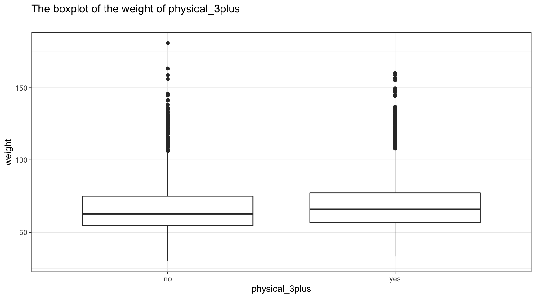 Inference:
Although almost similiar, there is a positive relationship between being physically active for at least 3 days a week and weight. The result is somehow counter-intuitive, since we thought that more exercise in children would reduce there weight. This might be explained by the reason that people who stay highly active take part of physically demanding sports like basket, football and similiar and have thus a higher percentage of muscle or are just bigger. One additional reason could be that kids who are slightly heavier are more incentivised to exercise more frequently.
Summary statistics for weight & confidence interval
#Apllying formula to weight
ci_yrbss_weight <- yrbss %>%
  filter(is.na(physical_3plus)==FALSE)%>%
  group_by(physical_3plus) %>%
  summarize(mean = mean(weight, na.rm=TRUE),
            sd = sd(weight, na.rm=TRUE),
            count = n(),
            t_critical = qt(0.975, count-1),
            se_diff = sd/sqrt(count),
            margin_of_error = t_critical * se_diff,
            weight_low = mean - margin_of_error,
            weight_high = mean + margin_of_error)

#Plotting results
kable(ci_yrbss_weight)| physical_3plus | mean | sd | count | t_critical | se_diff | margin_of_error | weight_low | weight_high |
|---|---|---|---|---|---|---|---|---|
| no | 66.7 | 17.6 | 4404 | 1.96 | 0.266 | 0.521 | 66.2 | 67.2 |
| yes | 68.4 | 16.5 | 8906 | 1.96 | 0.175 | 0.342 | 68.1 | 68.8 |
There is an observed mean difference of about 1.77kg (68.44 - 66.67), and we notice that the two confidence intervals do not overlap. It seems that the difference is statistically significant at 95% confidence.